How I got ready to make LaTeX files with RMarkdown
• • Reading time: 14 minutes
Last updated:
As an academic rooky I feel that I will eventually need to deal with LaTeX one way or another. However, I wonder whether I have to fully learn LaTeX if I’m already familiar with markdown, a way simpler formatting language. So I started searching the internet for solutions, and I think I found something useful for me.
LaTeX comes in a thousand flavours and each person will have a different preference. This post is therefore mostly recording what I have done for myself.
For context, I study psycholinguistics, where I put participants inside or in front of machines and do experiments with them (non-invasively, of course). So I already regularly deal with not-quire-small data sets in R, and share my workflow and results with supervisors and colleagues using RMarkdown. I also teach an introduction to statistics with R workshop where it’d be nice to prepare handouts that can include R codes and R results. I am also interested in sharing stuff I created with the community so it’d be nice to create pretty documentations. So when I learned that I can integrate LaTeX with RMarkdown, I immediately felt that this is where I want to start.
On this page, I will walk you step by step through how I set up everything to use RMarkdown to generate LaTeX files, including simple handouts, journal articles, and theses combined from multiple files.
On this page
- Prerequisites
- Write a simple pdf handout with RMarkdown
- Put together a long document using multiple RMarkdown files
- Write a journal article with RMarkdown
- Tips
Useful resources:
1. Prerequisites
My solution requires R, RStudio, and Pandoc.
Inside RStudio, install tinytex and TinyTeX by running install.packages("tinytex") and then tinytex::install_tinytex() in the console.
How it works:
- Create RMarkdown
.rmddocuments and write texts, codes, and generate results and plots.- Knit the .rmd file. During this process, knitr calls Pandoc, which will convert the document to .tex and generate a .pdf file accordingly.
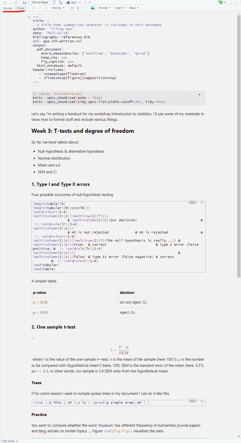
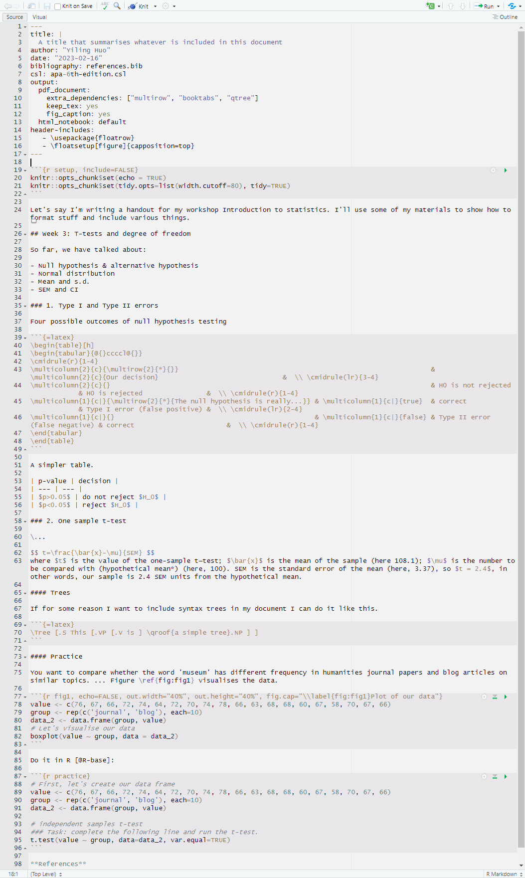
2. Write a simple pdf handout with RMarkdown
Create a new .rmd file: File - New File - RMarkdown…
Select Default Output Format: PDF.
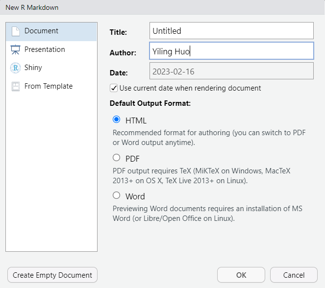
A .rmd file will be created, including some default text showing you how to write in markdown syntax and how to include R codes and plots.
The .rmd file contains two parts: a YAML header, which is enclosed in triple dashes on either side; and the text body. Inside the YAML header, we specify global variables for the document, and Pandoc will read the YAML header and adjust the LaTeX preamble accordingly during output.
We can edit this RMarkdown file and knit it by clicking the knit button. A PDF file will be created. Something like this:
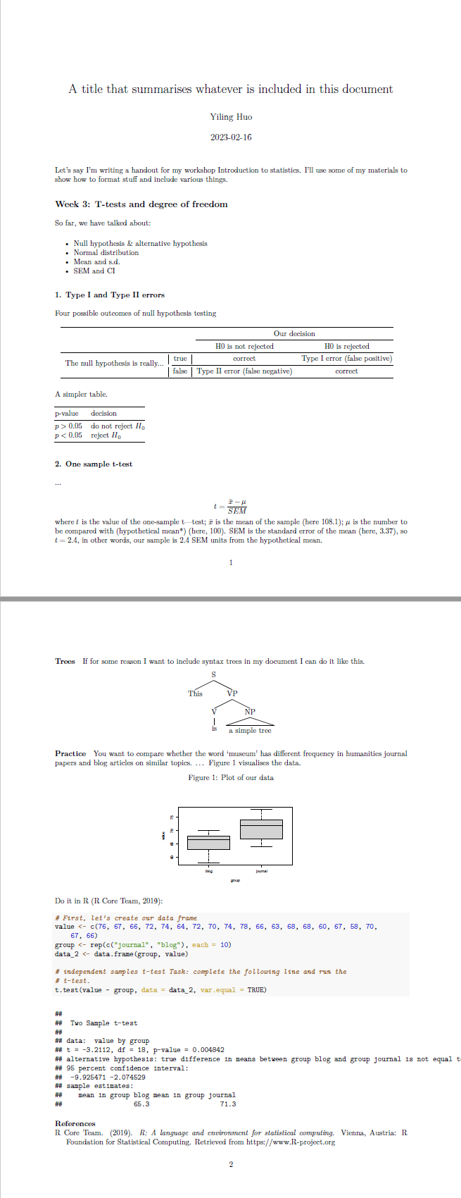
Writing your texts in RMarkdown:
Use markdown syntax to write your texts. For example, for your section title (heading level 1), you can write # 1. Introduction. To bold your text, write **text to bold**.
(If you have used markdown before, you may be inclined to include HTML codes for more detailed formatting. Unfortunately HTML will be ignored when Pandoc converts markdown to LaTeX. For anything that you instinctively want to use HTML, just google a LaTeX solution.)
Including R and/or other languages codes and results:
In RStudio, you can include a R code chunk in your document by pressing Ctrl + Alt + I (Mac: Cmd + Option + I); or clicking the Add Chunk button in the toolbar; or simply typing:
```{r}

```
You can name your chunk by typing after {r, separated by a space: {r chunk_name}. Chunk options are separated by comma: {r chunk_name, echo = TRUE, message = FALSE, warning = FALSE}. Chunk options control whether and how the code and the results are shown in your output document. You can find a list of all possible chunk options at the knitr documentation.
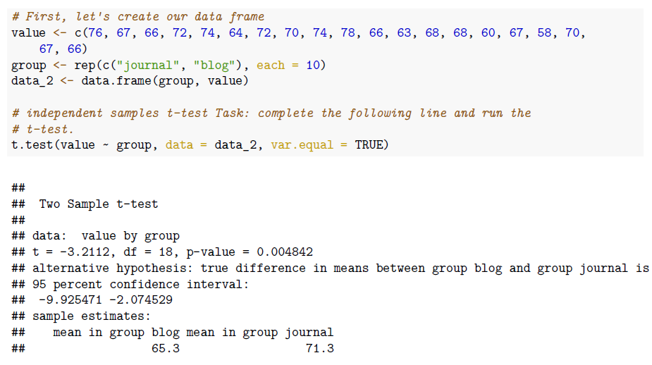
```{r}
# First, let's create our data frame
value <- c(76, 67, 66, 72, 74, 64, 72, 70, 74, 78, 66, 63, 68, 68, 60, 67, 58, 70, 67, 66)
group <- rep(c('journal', 'blog'), each=10)
data_2 <- data.frame(group, value)

# independent samples t-test
### Task: complete the following line and run the t-test.
t.test(value ~ group, data=data_2, var.equal=TRUE)
```
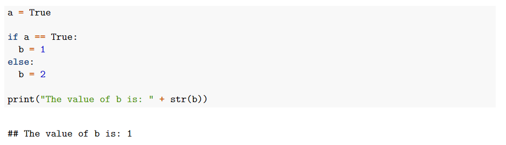
RMarkdown supports many languages other than R through the knitr package. A list of supported languages can be found here. For example, if I want to include a chunk of python code:
```{python}
a = True

if a == True:
  b = 1
else:
  b = 2

print("The value of b is: " + str(b))
```
Including figures and plots:
method 1: include plots as images
RMarkdown allows including external images quite easily. If you have been working in other R project and generated R plots, you can save the plots as PDF first, and include the PDF image in your .rmd document. (Other image formats are also fine, and may be preferred if your have complex plots. PDF’s advantage is it’s vector-based, so can be directly sent to your editors for publishing.)
In your other R project, if you have base R plots:
# dimensions are in inches. width = 7.25 satisfies most journal requirements.

# create pdf file
pdf("file_name.pdf", width = 7.25, height = 5)
# your code for the plot
boxplot(value ~ group, data = data_2)
# close the pdf file
dev.off()
If you have ggplot2 plots:
pdf("file_name.pdf", width = 7.25, height = 5)
print(ggplot_object)
dev.off()
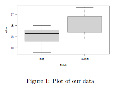
In your RMarkdown file, you can include your figures in a R code chunk. Specify chunk options, then use knitr to include the plot:
```{r, echo=FALSE, out.width="40%", fig.align="center", fig.cap="\\label{figure-label}Plot of our data"}

knitr::include_graphics("./file_name.pdf")
```
Put your PDF figure in the same folder as your RMarkdown file, or specify the relative path to your figure such as (./path/to/figure/figure.pdf).
The above line includes some common LaTeX figure configurations you can directly add to your RMarkdown file: \label{figure-name} allows you to label your figure for cross referencing, out.width=40% allows you to control the size of the figure.
Alternatively, you can include images using Markdown syntax:
{width=40%}
Other images can also be included in these manners.
method 2: include R plots as R object
Another method is to directly include your R plots as a R object. In your other R project, run:
saveRDS(object_name, "./file_name.rds")
Note that your plot cannot refer to data frames other than the one originally mentioned in the main function. For example, the following plot CANNOT be successfully read:
plot <- ggplot(data_frame_1, aes(x=a, y=b)) +
    	geom_bar(stat='stat') +
        goem_point(data=data_frame_2, aes(x=mean(V1), y=0.5)) # the point refers to data from another data frame
In your RMarkdown file:
```{r, echo=FALSE, out.width="40%", out.height="40%", fig.align="center", fig.cap="\\label{fig:fig1}Plot of our data"}

plot <- readRDS("rile_name.rds")
plot
```
Including tables:
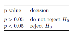
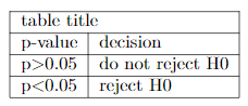
method 1: markdown tables
Markdown allows you to create simple tables. Use pipes (|) to create cells and use multiple hyphens (—) to separate the header from other cells. More details here. For example:
| p-value | decision |
| --- | --- |
| $p>0.05$ | do not reject $H_0$ |
| $p<0.05$ | reject $H_0$ |
method 2: LaTeX tables
If your table goes beyond the capacity of markdown, for example, if you want to merge cells, you can directly include a LaTeX table as a LaTeX chunk. Don’t worry about not knowing LaTeX, there are many online tools such as tablesgenerator that allow you to generate LaTeX code for tables. Simply copy and paste the codes in your document. You can also make it a code chunk. For example:
```{=latex}
\begin{table}[]
\begin{tabular}{lllll}
\cline{1-2}
\multicolumn{2}{|l|}{table title}                                          \\ \cline{1-2}
\multicolumn{1}{|l|}{p-value}             & \multicolumn{1}{l|}{decision}  \\ \cline{1-2}
\multicolumn{1}{|l|}{p\textgreater{}0.05} & \multicolumn{1}{l|}{do not reject H0} \\ \cline{1-2}
\multicolumn{1}{|l|}{p\textless{}0.05}    & \multicolumn{1}{l|}{reject H0} \\ \cline{1-2}
\end{tabular}
\end{table}
```
The table generator may tell you to add packages to your document preamble, you can do so in the YAML header at the beginning of your document. For example:
---
output:
  pdf_document:
    extra_dependencies: ["multirow", "booktabs"]
---
Including math equations:
Inline mathematics are enclosed in dollar signs on both sides. No need to put spaces between the dollar signs and your equation. For example, $E=mc^2$ will render
Use double dollar signs for displayed equations. For example, $$E=mc^2$$ will render:
A list of how to write common mathematical notations can be found here.
References and citations:
Citing others’ work:
Citations can be managed simply. To begin, you can put all of your citations in .bib format in a .bib file. (To create a new .bib file, simply create a new .txt file then change the extension.) Put the .bib file in the same folder as your RMarkdown file. Specify your reference file in the YAML header:
---
bibliography: references.bib
---
Or use multiple bib files:
---
bibliography: ["references1.bib", "references2.bib"]
---
From your source material, simply look for BibTeX format citation, then copy and paste the content to the .bib file. Like this:
@article{kutas1984brain,
  title={Brain potentials during reading reflect word expectancy and semantic association},
  author={Kutas, Marta and Hillyard, Steven A},
  journal={Nature},
  volume={307},
  number={5947},
  pages={161--163},
  year={1984},
  publisher={Nature Publishing Group UK London}
}

@book{chomsky2014minimalist,
  title={The minimalist program},
  author={Chomsky, Noam},
  year={2014},
  publisher={MIT press}
}
Popular citation management apps should have an option to export a .bib file from your citation pool, too. For example, I use Mendeley to manage my references. In Mendeley, you can export a .bib file by selecting citations you want to export and clicking File - Export. This will export a .bib file containing information of all the documents you selected.
Note that the first argument of a BibTex citation entry is the key, such as kutas1984brain and chomsky2014minimalist. To cite an item in-text, simply write @key. To enclose citation in parentheses, write [@key]. To cite multiple items in one parentheses, write [@key1; @key2; @key3]. You can also have normal text within the citation parentheses, such as [e.g., @key] or [for a review, see @key]. A more detailed explanation can be found here.
Citation style is managed by .csl files. Download the desired .csl file here and put it in the same folder. Use reference-section-title: in the front matter to give your reference section a title.
---
bibliography: references.bib
csl: apa-6th-edition.csl
reference-section-title: "References"
---
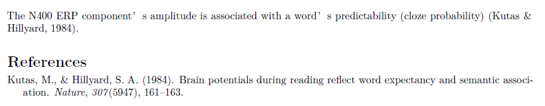
The N400 ERP component's amplitude is associated with a word's predictability (cloze probability) [@kutas1984brain].
If you are citing multiple papers from the same author(s), you can write down the authors’ name manually and use a minus (-) sign before the @ sign to suppress the authors’ name in the citation:
Lew-Williams & Fernald [-@lew2007young; -@lew2010real] used the visual world paradigm.

Labelling and cross referencing sections, tables, and figures:
Labelling and referencing can be managed by some simple LaTeX syntax.
To label a section in your document, add {#id} to the end of your section header. To reference this section, write \ref{id}.
## Neuronal Cytoarchitecture {#cyto}

In section \ref{cyto}, we talk about neuronal cytoarchitecture.
To label and reference a markdown table:
| Header 1 | Header 2 |
| --- | --- |
| Cell content 1 | Cell content 2 |

Table: \label{tablekey} Your Caption.

In Table \ref{tablekey}, we can learn about how to reference tables.

To label and reference a LaTeX table, include lines \caption{} and \label{} after line \begin{table}[]. Online table generators can take care of this.
```{=latex}
\begin{table}[h]
\caption{Caption}
\label{tablekey2}
\centering
\begin{tabular}{@{}lllll@{}}
\cmidrule(r){1-2}
\multicolumn{2}{l}{Header} \\ \cmidrule(r){1-2}
Cell 1       & Cell 2      \\ \cmidrule(r){1-2}
\end{tabular}
\end{table}
```

In Table \ref{tablekey2}, we can learn about how to reference tables.
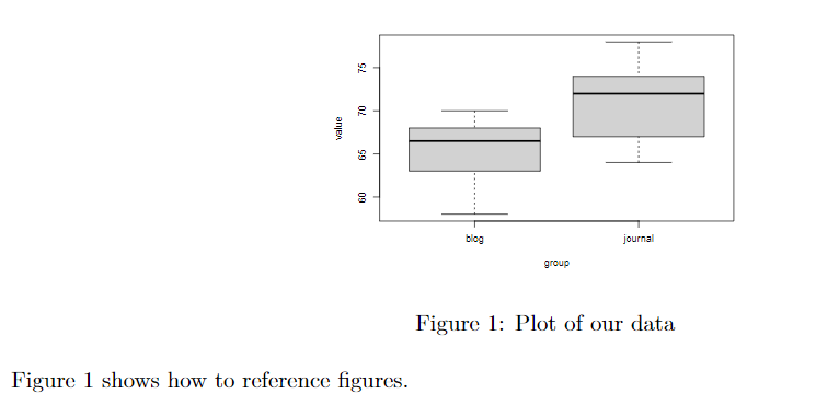
To label and reference a figure, include \label{} in your figure caption:
```{r, echo=FALSE, out.width="40%", out.height="40%", fig.align="center", fig.cap="\\label{figkey}Plot of our data"}

knitr::include_graphics("./file_name.pdf")
```

Figure \ref{figkey} shows how to reference figures.
Or
{width=40%}
Figure \ref{figkey} shows how to reference figures.
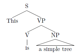
Including syntax trees:
I work closely with linguistics, so one day I may need to include syntax trees in my documents.
Syntax trees can be easily included as LaTeX codes using the packages such as Forest or Qtree. Here I will show a simple example using Qtree. Include the package in the YAML header:
---
output:
  pdf_document:
    extra_dependencies: ["qtree"]
---
The Qtree package allows users to write syntax trees in phrase marker style (with some simplest LaTeX syntax), and will generate trees during output:
```{=latex}
\Tree [.S This [.VP [.V is ] \qroof{a simple tree}.NP ] ]
```
Including linguistic examples:
It appears that including linguistic examples can only be done in LaTeX syntax. So in this section I will have to go against what I was claiming in the beginning of this tutorial, and talk about how to include linguistic examples using LaTeX.
There are several LaTeX packages that deal with linguistic examples, in this tutorial I will use bg4e.
Include the bg4e package in the YAML header:
output:
  pdf_document:
    extra_dependencies: ["gb4e"]
The simplest linguistic example using bg4e looks like this:
```{=latex}
\begin{exe}
\ex
\label{label-name}
This is not a pipe.
\end{exe}
```

Reference the examples using \label{label-name} and \ref{label-name}.
The bg4e package allows more formatting of examples, such as ungrammatical marking, listing, glosses, etc. You can refer to their documentation for more details.
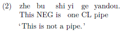
```{=latex}
\begin{exe}
\ex
\label{label-name}
\gll zhe bu shi yi ge yandou. \\
This NEG is one CL pipe\\
\trans ‘This is not a pipe.’
\end{exe}
```
Including Chinese and Japanese characters
The easiest way to include some Chinese and Japanese characters in an otherwise English document is using XeTeX’s xeCJK package. This package also supports Korean characters, with some font settings, details here and here. To use this package, the PDF engine has to be set to xelatex.
In your YAML header, specify the PDF engine, and use the xeCJK package:
---
output:
   pdf_document:
       latex_engine: xelatex
       extra_dependencies: ["xeCJK"]
---
Then you can freely include the characters in your document:
For example, my document needs these characters:

- 用汉语说你好
- 日本語でこんにちは
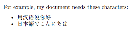
Note that your PC needs to have fonts for these languages installed.
3. Put together a long document using multiple RMarkdown files
When you are preparing a long document, you might prefer to write each section in a different RMarkdown file. You can easily do that and put the long file together using an index (main structure) RMarkdown file. To include other Rmd files as child files:
```{r, child=c('one.Rmd', 'two.Rmd')}
```
For example, my index RMarkdown file may look like this:
---
title: "Sample"
author: "Yiling Huo"
date: \today
bibliography: ref.bib
csl: apa.csl
reference-section-title: "References"
output:
    pdf_document:
        number_sections: true
---

# Introduction

```{r, child='intro.Rmd'}
```

# Experiment 1

```{r, child=c('exp1_intro.Rmd', 'exp1_methods.Rmd', 'exp1_dis.Rmd')}
```

# General Discussion

```{r, child='general_dis.Rmd'}
```
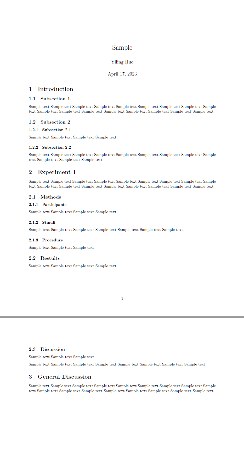
A sample child document exp1_methods.Rmd:
## Methods

### Participants

Sample text Sample text Sample text Sample text

### Stmuli

Sample text Sample text Sample text Sample text Sample text Sample text Sample text

### Procedure

Sample text Sample text Sample text

## Restults

Sample text Sample text Sample text Sample text

## Discussion

Sample text Sample text Sample text
When I knit the parent RMarkdown, the output looks like this:
4. Write a journal article with RMarkdown
You can use the rticles package to easily use templates from a large number of publishers.
In R console, run install.packages("rticles").
In File - New File - RMarkdown…, select using templates, and select your target publisher. Replace the template content with your content, and your document will be the format required by your target publisher.
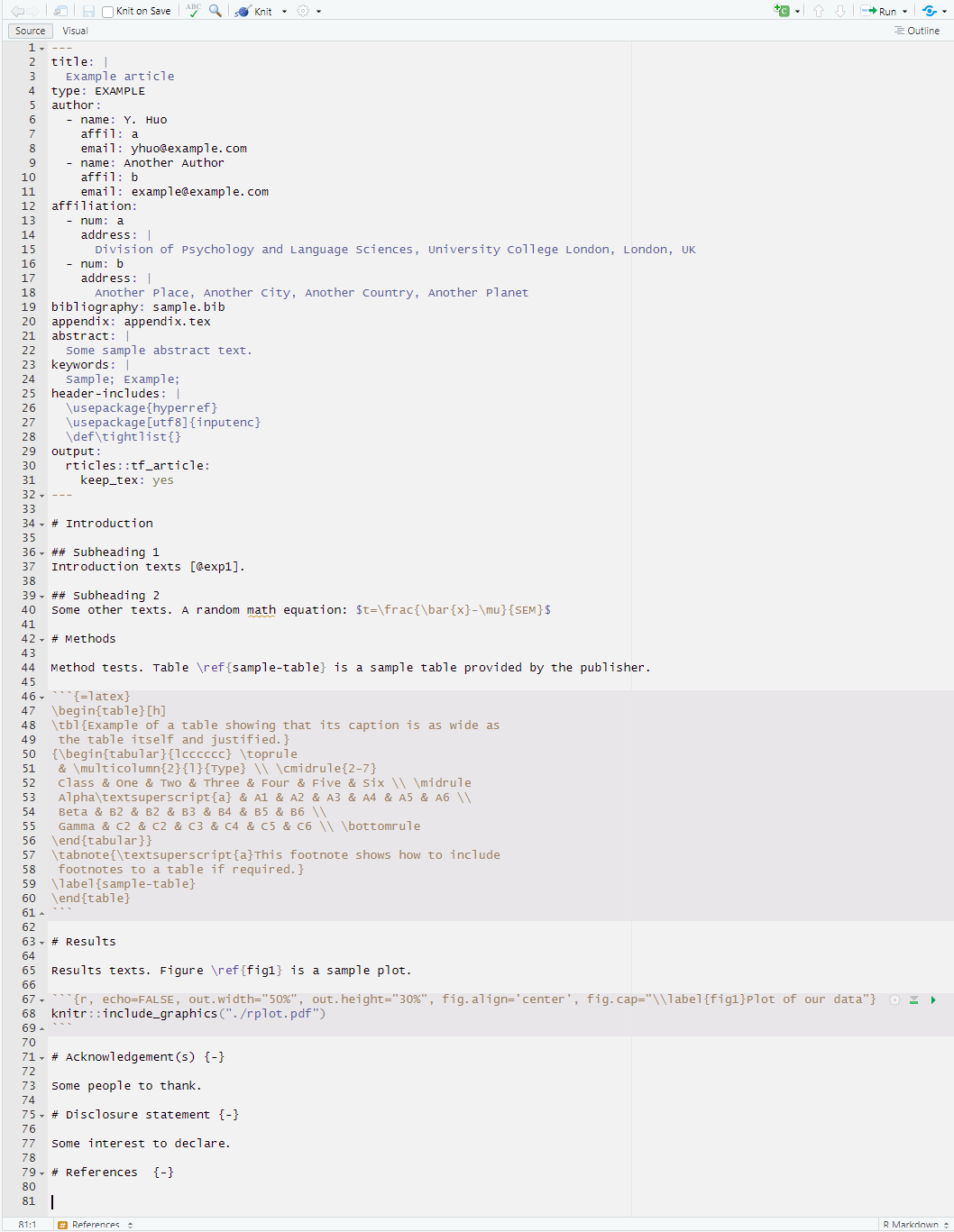
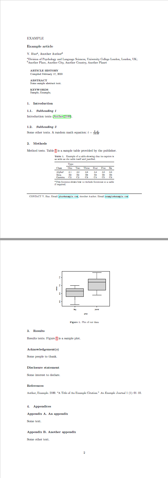
For example, I have created an example using the Taylor & Francis Journal Article template:
5. Tips
Keep_tex: yes
Inside the YAML header, under output, set keep_tex: to yes to generate .tex files alongside PDF files.
---
output:
  pdf_document:
    keep_tex: yes
---
Use RStudio’s visual editor
You may find it easier to edit texts using RStudio’s MS Word style visual editor. In RStudio, turn on visual editor at the toolbar: